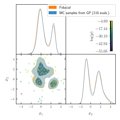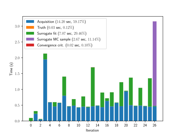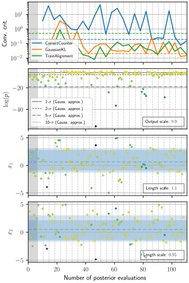
Advanced example

Note

The code for the example is available at ../../examples/advanced_example.ipynb and ../../examples/advanced_example.py

The goal of this example is to show how to pass to the Runner options for the different components, as well as to discuss how GPry can be tuned for more complicated posteriors.

As before, let us define our likelihood, here as a gaussian mixture with 4 components:

import numpy as np
from scipy.special import logsumexp
from scipy.stats import multivariate_normal

means = [
    [-0.5, -0.5],
    [0, 2],
    [0.5, 1.5],
    [2.5, -1]]
covs = [
    [[0.25, -0.1], [-0.1, 0.25]],
    [[0.25, 0.], [0., 1]],
    [[1, -0.1], [-0.1, 0.25]],
    [[0.15, 0.05], [0.05, 0.15]],]

rvs = [multivariate_normal(m, c) for m, c in zip(means, covs)]

def logLkl(x, y):
    return logsumexp([rv.logpdf(np.array([x, y]).T) for rv in rvs])

bounds = [[-5, 5], [-5, 5]]

We will draw some samples from the true distribution to use them as a fiducial reference in the runner. (This is of course optional.)

# Draw samples
n_samples = 100000

indices = np.random.choice(len(rvs), n_samples)
samples = np.empty(shape=(n_samples, 2))
for i, rv in enumerate(rvs):
    j_i = np.where(indices == i)[0]
    samples[j_i] = rv.rvs(size=len(j_i))

# Let's plot the likelihood
from getdist import MCSamples, plots

mcsamples = MCSamples(samples=samples)
g = plots.get_subplot_plotter()
g.triangle_plot([mcsamples], filled=True)

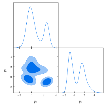
Let us now create the Runner object.

We expect the likelihood to be multimodal, so we will tune some parameters to explore the distribution more efficiently and ensure convergence without missing any modes (e.g. by making GPry more exploratory).

Below you can see the general structure for specifying options for sub-modules such as the surrogate model, the acquisition engine, and the convergence criteria. For example, for the acquisition engine we find in the Runner documentation that it is set with the gp_acquisition keyword. Then we look into the documentation of the gp_acquisition module to find the arguments that can be passed when initializing the NORA class, and specify them as gp_acquisition={"NORA": {option: value}}.

from gpry import Runner
checkpoint = "output/adv"

runner = Runner(
    logLkl,
    bounds,
    options={
        # If there is multimodality, we are more likely to be
        # exploring simultaneously a couple of interesting areas
        # so we can evaluate more points per iteration
        "n_points_per_acq": "2d",
        # We will probably need more training samples than default
        # to represent a complicated posterior surface
        "max_total": 400},
    surrogate={
        "regressor": {
            # We want to adapt hyperparameters more often, to make
            # it more likely to converge earlier
            "n_restarts_optimizer": 20}},
    gp_acquisition={
        "NORA": {
            # We want to make the acquisition function more
            # exploratory (higher zeta_scaling)
            "acq_func": {"LogExp": {"zeta_scaling": 1.1}},
            # We want to re-run the nested sampler exploration as
            # often as possible, because we expect frequent changes
            "mc_every": 1}},
    convergence_criterion={
        # We want to make the CorrectCounter criterion necessary,
        # not just sufficient, so that it detects when a new region
        # is being explored. But we can also relax it a bit.
        "CorrectCounter": {"policy": "n", "reltol": 0.05, "abstol": "0.05s"},
        "GaussianKL": {"policy": "n"},
        "TrainAlignment": {"policy": "n"},},
    mc={
        # In the final MC run, we want more live points for a
        # better exploration of all the modes
        "nested": {"nlive": "100d"}},
    # Just for diagnostics. It will severely slow down the run if uncommented
    # plots={
    #     # Let's do a corner plot per iteration
    #     "corner": True, "timing": False, "convergence": False,
    #     "trace": False, "slices": False, "ext": "png"},
    checkpoint=checkpoint,
    load_checkpoint="overwrite")

runner.set_fiducial_mc(samples)

And now we run it. This will take a little while, especially if the plots kwarg has been uncommented.

runner.run()
runner.plot_progress()