How does GPry work#
GPry creates an interpolating model of the log-posterior density function. It does so using the least amount of evaluations possible. The locations in parameter space of these evaluations are chosen sequentially, so that they maximise the amount of information that can be obtained by evaluating the posterior there.
Here we explain some of the key aspects of the GPry algorithm. Most of what follows is not exclusive to GPry, but typical in active learning approaches.
Active learning of a Gaussian Process#
GPry does not need any pre-training: it trains its surrogate model at run time by selecting optimal evaluation locations. The process of selecting these optimal locations based on current information is commonly known as active learning. It involves finding the maximum of an acquisition function measuring the amount of information about the true model expected to be gained by evaluating it at a given point. Acquisition functions must manage a good balance between exploration (getting an overall-good model of the true function) versus exploitation (prioritising a better modelling of the true function where its value is the highest). The default acquisition function used by GPry is described in [TODO: reference]
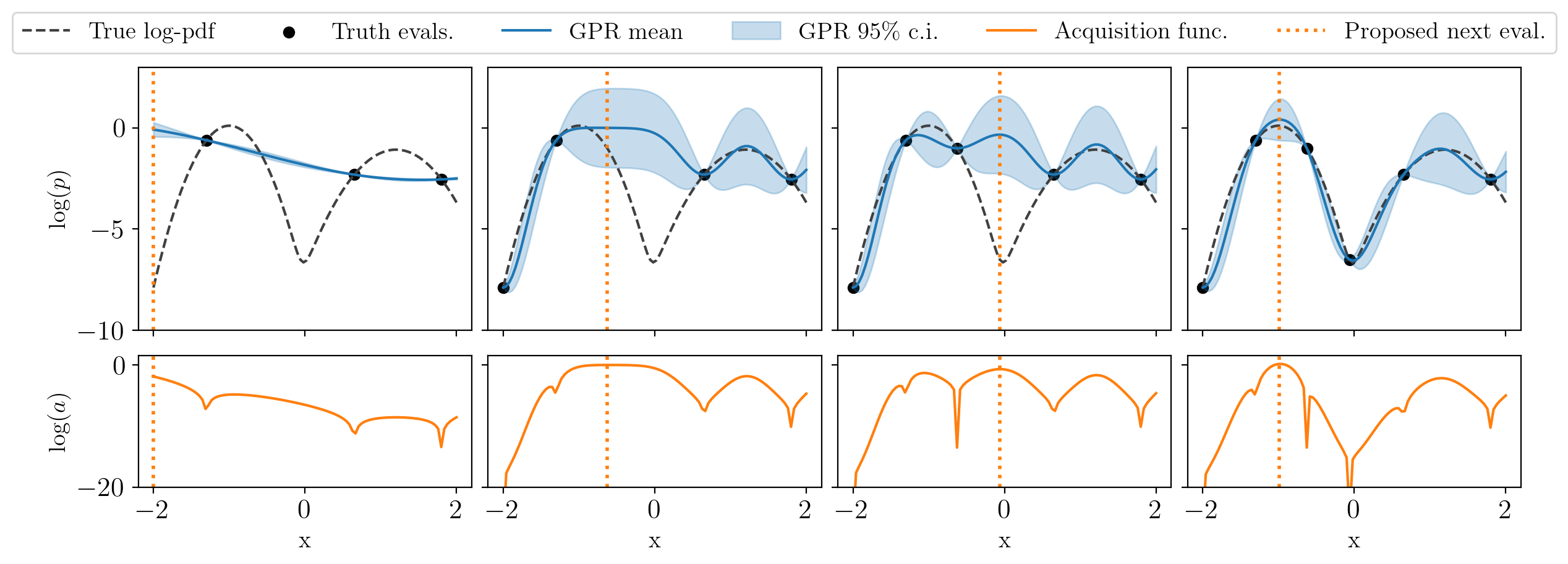
You can see the way active learning works in the following figure: the top plots show the current GP model, and the bottom ones the value of the acquisition function (for this simple example, the GP standard deviation times the exponential of the double of the GP mean); every column is an iteration of the algorithm. Notice how at every step an evaluation of the true function at the previous maximum of the acquisition function has been added:
Note
This aspect of GPry is one of the main difference with amortised approaches, such as forward-modelling (or simulation-based) inference: the latter can produce inference at very low cost in exchange for some usually-costly pre-training; instead, the cost of inference in active learning approaches is higher (due both to the need for evaluating the true posterior at least a few times, and the overhead from active sampling), but they do not need pre-training.
Parallelising truth evaluation with kriging-believer#
The active learning approach described above is sequential: one candidate is proposed for evaluation of the true posterior at a time. But being this evaluation often the slowest step, if one has sufficient computational resources available to perform \(n\) posterior evaluations in parallel it would be desirable to obtain not just the next optimal location, but the next \(n\) optimal ones.
However, simultaneously optimizing the acquisition function for a set of candidate locations is not a trivial problem: each of the candidates modifies the landscape of the acquisition function for the rest, so that we cannot simply assume that a set of local maxima is a viable solution.
But there is one way to give up some effectiveness (total information gained) of the solution in exchange for the possibility to turn this into a sequential problem: we can find the global maximum, assume an evaluation of the true model there, to which the mean of the GP is assigned, create with it an augmented model, and repeat this procedure using the augmented model, as many times as desired. This approach is called kriging-believer (KB), and though suboptimal, it at least includes the effect of the exploration term of the acquisition function, reducing the amount of redundant information with respect to a naive multiple-candidate solution.
Obviously, this procedure only makes sense up to a certain amount of iterations, or we risk assuming completely false information about the model. In GPry, we recommend at most a number of KB steps equals to the dimensionality of the problem (times some factor smaller or equal the number of expected posterior modes, if more than one).
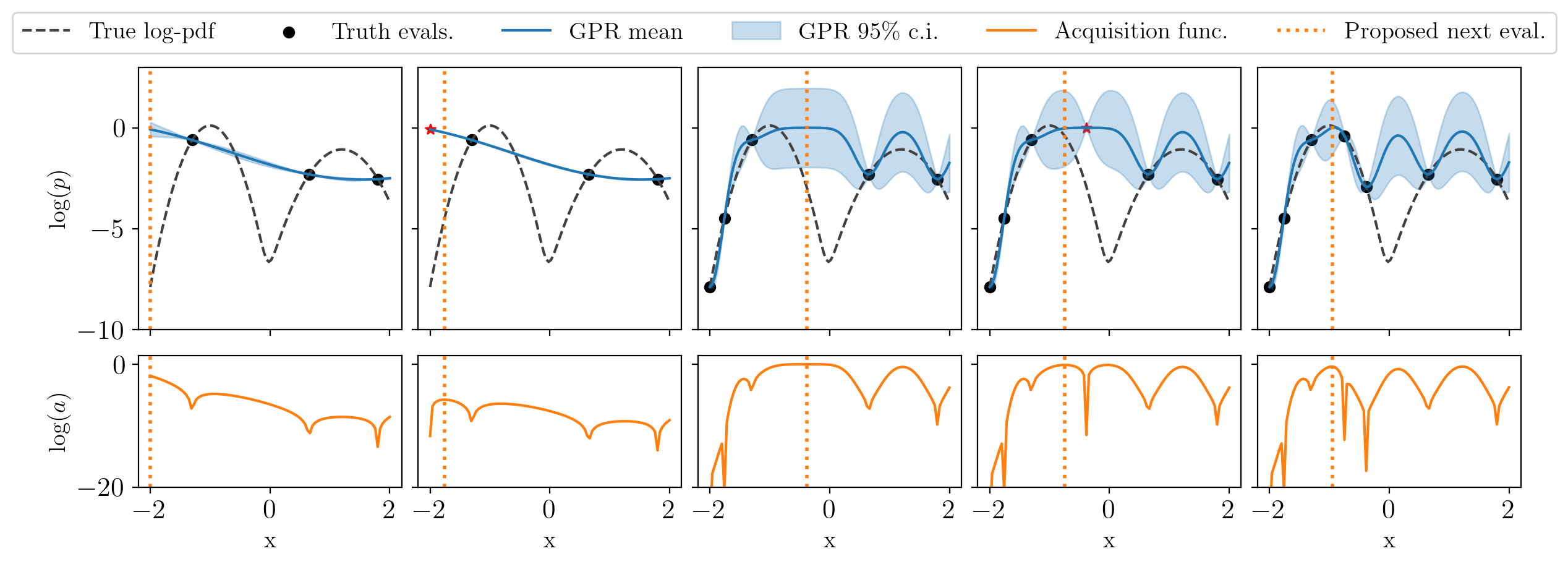
In the following figure, to be compared with the one above, we only evaluate the posterior every two steps, the red stars in being the temporary kriging-believer evaluations that will be assigned their true values in the next iteration.
Acquisition mechanism#
NORA vs BatchOpt
Hyperparameter fit#
Convergence check#
MCMC from GP#
The algorithm, putting everything together#
Flow-chart
From old README#
Unlike algorithms like MCMC which sample a posterior distribution GPry is designed to interpolate it using Gaussian Process regression and active sampling. This converges to the posterior shape requiring much fewer posterior samples than sampling algorithms because it sets a prior on the functional shape of the posterior. This doesn’t mean that your posterior has to have a certain shape but rather that we assume that the posterior is a continuous, differentiable function which has a single characteristic length scale along each dimension (don’t take this too literally though. It will still work with many likelihoods which do not have a single characteristic length-scale at all!) Furthermore GPry implements a number of tricks to mitigate some of the pitfalls associated with interpolating functions with GPs. The most important ones are: - A novel acquisition function for efficient sampling of the parameter space. This procedure is inspired by Bayesian optimization. - A batch acquisition algorithm which enables evaluating the likelihood/posterior in parallel using multiple cores. This is based on the Kriging-believer algorithm. A nice bonus is that it also decreases the time for fitting the GP’s hyperparameters. - In order to prevent sampling regions which fall well outside the 2- σ contours and account for the fact that many theory codes just return 0 far away from the fiducial values instead of computing the actual likelihood (which leads to - ∞ in the log-posterior) we shrink the prior using an SVM classifier to divide the parameter space into a “finite” region of interest and an “infinite” (uninteresting) region. - Instead of simply optimizing the acquisition function we created the **N**ested sampling **O**ptimization for **R**anked **A**cquisition algorithm for parallelizing the acquisition procedure and gaining robustness with regards to the highly multimodal nature of the acquisition function.
The requirements that your likelihood/posterior has to fulfil in order for this algorithm to be efficient and give correct results are as follows:
The likelihood/posterior should be smooth (continuous) and you should know how smooth (how many times differentiable).
(there can be a little noise, but it must be deterministic!!!!)
The likelihood/posterior evaluation should be slow. What slow means depends on the number of dimensions and expected shape of the posterior distribution but as a rule of thumb, if your MCMC takes longer to converge than you’re willing to wait you should give it a shot.
The likelihood should be low-dimensional (d<20 as a rule of thumb). In higher dimensions you might still gain considerable improvements in speed if your likelihood is sufficiently slow but the computational overhead of the algorithm increases considerably.
Like every other sampler GPry isn’t perfect and has some limitations: - GPs don’t scale well with the number of training samples as training the GP involves inverting a kernel matrix. Unfortunately the computational complexity of this inversion scales with the number of training samples cubed. This means that as the number of training samples required grows, the overhead of the algorithm increases considerably. - While we tested GPry on mildly multimodal posterior distributions it is not a supported feature and should be used with caution. The algorithm is fairly greedy and can easily miss a mode, especially if the separation between modes is large. - The algorithm is generally robust towards “weirdly” shaped posterior distributions, however the structure of the kernel still assumes a single characteristic correlation length. This means that in very pathological cases (for instance a very wide distribution with a tiny spike in it) GPry will struggle to capture the mode correctly. - This code is novel and hasn’t profited from years of user feedback and maintenance. Bugs can (and probably will) occur. If you find any please report them to us!
We are actively working on mitigating some of those issues and we will keep on developing this code so look out for new versions!