Advanced example to using GPry

Warning

This code for this example is probably outdated at the moment, but the basics are as presented. It will be updated soon.

This example shows some of the ways in which it is possible to customize the Bayesian optimization loop. This will be done using a less standard (non-gaussian) likelihood and we will walk through the modules and their functionalities one by one.

Warning

Mind that this example is really just meant to show off how one can change things in the BO loop. For the vast majority of posterior distribution which are compatible with GPry the standard parameters will work just fine and probably produce the best results.

Therefore it is usually a good idea to keep things as standard except if you want to play around with the code and/or have very good reasons to customize things (i.e. when you know that your posterior distribution isn’t particularly smooth).

Introduction

In this example we use a curved 2d variation of a guassian with the curving degeneracy being generated by a 8-degree polynomial in the exponent. It has the following (un-normalized) likelihood:

\[y(x) \sim \exp(-25\cdot(0.45-x_1)^2 - 20\cdot(x_2/2-x_1^4)^2)\]

with \(x=(x_1, x_2)^T\).

Since our GP maps the log-posterior and uses the log-likelihood as input the likelihood function looks something like this:

def log_lkl(x_1, x_2):
    return  -(10*(0.45-x_1))**2./4. - (20*(x_2/4.-x_1**4.))**2.

We could map this likelihood using the standard parameters of the run.run() function, which would recover the correct marginals. Since the goal of this example is to showcase the ways in which the BO loop can be modified we will change things though.

In order to make this as easy to understand as possible I will walk you through every step of building the model, running it and plotting. I will reference the individual modules where they are used. They contain further detailed documentation on how to implement the different custom options as well as on how to create custom classes which inherit from the base classes.

The GPry algorithm needs 5 basic building blocks to learn the shape of a posterior distribution:

• The model which contains the log-likelihood and the prior.

• The GP regressor which is used to interpolate the posterior.

• The Acquisition object which determines the next sampling locations in each step of the Bayesian optimization loop.

• The Convergence criterion which determines when the GP has converged to the shape of the posterior distribution and and hence the Bayesian optimization loop should be stopped.

• The options dictionary setting the parameters for the actualy Bayesian optimization.

This is followed by a call to the run function which

The Model

It is generally a good idea to define the model (i.e. the prior) first. For this we need to create a Cobaya model object which contains the prior and log-likelihood:

from cobaya.model import get_model
info = {"likelihood": {"curved_degeneracy": log_lkl}}
info["params"] = {
    "x_1": {"prior": {"min": -0.5, "max": 1.5}},
    "x_2": {"prior": {"min": -0.5, "max": 2.}}
    }
model = get_model(info)

For building the parts of our BO-loop we will need the dimensionality and the prior bounds of our model which we get in the following way:

n_d = model.prior.d()
prior_bounds = model.prior.bounds()

If you have unbounded priors (like a normal distribution) use the keyword confidence_for_unbounded (see here)

The GP Regressor

The first part of our model which we have to define is the GP regressor. This object also contains the kernel. It’s hyperparameters are optimized in every iteration of the BO loop.

Kernel

Even though the standard RBF kernel would work well enough for this likelihood we will spice things up a bit by constructing a custom kernel which consists of a Matèrn kernel with \(\nu=5/2\) multiplied with a Constant kernel (and non-dynamic, i.e. fixed bounds):

from gpry.kernels import Matern, ConstantKernel as C
kernel = C(1.0, (1e-3, 1e3)) * Matern([0.1]*n_d, [[1e-5, 1e5]]*n_d, nu=2.5)

For details on the kernel construction see kernels.

Note

For kernels containing length-scales (i.e. RBF and Matèrn kernel) the bounds can automatically be adjusted according to the size of the prior. For this you need to pass "dynamic" for the bounds parameter and provide prior bounds to the kernel.

GP Regressor

Now it’s time to construct the actual GP regressor object. In addition to the kernel this sets all the variables associated to the optimization procedure of the hyperparameters as well as how the data is preprocessed. Since we want our model to converge to the correct hyperparameters more robustly we increase n_restarts_optimizer (the number of restarts of the optimizer for the GP’s hyperparameters) to 20.

Furthermore it is generally a good idea to scale the parameter space to make it a unit hypercube as is done as standard when calling the run.run() function:

from gpry.gpr import GaussianProcessRegressor
from gpry.preprocessing import Normalize_bounds, Normalize_y
gpr = GaussianProcessRegressor(
    kernel=kernel,
    n_restarts_optimizer=20,
    preprocessing_X=Normalize_bounds(prior_bounds)
    )

Details can be found in the gpr and preprocessing modules.

Note

The SVM which divides posterior samples into a finite and an infinite category is part of the GP regressor. I advise keeping it as standard but there are options for changing it. For this see the svm module.

Note

We did not process the target values of the posterior distribution before fitting the GP. In our example this is not a bit problem as the range of the log-likelihood is relatively modest. If your log-likelihood ranges several orders of magnitude (i.e. when you have a big prior) it is usually a good idea to scale your target values using preprocessing.Normalize_y

Note

The likelihood/posterior samples from some theory codes may contain some form of noise. If this is the case you might have to increase the noise_level parameter in the GP (set to 1e-2 as standard) to the numerical noise of your posterior samples.

Acquisition

The acquisition module contains both the acquisition function as well as the optimization procedure for it. It operates similarly to the GP regressor module.

Acquisition function

The acquisition function is the centerpiece of the Bayesion optimization procedure and decides which point the algorithm samples next. The acquisition_functions module has multiple inbuilt acquisition functions as well as building blocks for custom acquistion functions which can be constructed using the + and * operators. Since it tends to perform best we will use the standard acquisition_functions.Log_exp acquisition function with a \(\zeta\) value of 0.05 to encourage exploration (as we know that the shape of the posterior distribution is not very gaussian):

from gpry.acquisition_functions import Log_exp
af = Log_exp(zeta=0.1)

Then it is time for the actual GP Acquisition. For this we need to build our instance of the gp_acquisition.GPAcquisition class which also takes the acquisition function. Furthermore it needs the prior bounds so it knows which volume to sample in. Furthermore like with the GP regressor it is usually a good idea to scale the prior bounds to a unit hypercube (assuming that the mode occupies roughly the same portion of the prior in each dimension) as the optimizer tends to struggle with very different scales across different dimensions:

from gpry.gp_acquisition import GPAcquisition
acq = GPAcquisition(
    prior_bounds,
    acq_func=af,
    n_restarts_optimizer=10,
    preprocessing_X=Normalize_bounds(prior_bounds)
    )

Convergence

Next we need to set how the algorithm determines whether it has converged to the correct posterior distribution. This is set using the convergence module which offers a base convergence.ConvergenceCriterion class of which several inbuilt convergence criteria inherit. Using this base class it is also possible to construct custom convergence criteria.

The standard convergence.CorrectCounter convergence criterion works best in most cases and I highly recommend using it. For educational purposes we will use convergence.GaussianKL which computes the KL divergence assuming that the target distribution is a multivariate gaussian. The KL divergence is computed by running a short MCMC chain of the GP and estimating the mean and covariance matrix of the distribution from it. This convergence criterion is considerably slower than convergence.CorrectCounter but it can be useful as it provides a more direct statistical measure of convergence.

All convergence criteria are passed a prior object which is part of the model instance and an options dict. The options that can be set depend on the choice of the convergence criterion. In our case we set the KL divergence between steps that we want to reach to \(10^{-2}\):

from gpry.convergence import GaussianKL
conv = GaussianKL(model.prior, {"limit": 1e-2})

Training parameters

The training parameters which control the bayesian optimization loop are set in the options dict. There we can also manually set the number of Kriging believer steps per iteration and the maximum number of samples that the algorithm draws from the posterior distribution before failing:

options = {"max_init": 100, "max_points": 200,
           "n_initial": 8, "n_points_per_acq": 2}

Note

If "n_points_per_acq" isn’t set it defaults to the number of MPI processes to utilize the parallel evaluation of the posterior with Kriging believer.

Training

Like in the simple example we simply create a run.Runner object and use the run.Runner.run() method to run the Bayesian optimization loop. The only difference is that we now have to pass our custom objects to the run.Runner at initialization. To spice things up a bit we also now choose the "resume" checkpoint policy meaning that the run is automatically resumed from the checkpoint files if they exist:

from gpry.run import Runner
checkpoint = "output/advanced"
runner = Runner(
    model, gpr=gpr, gp_acquisition=acq, convergence_criterion=conv, options=options,
    checkpoint=checkpoint, load_checkpoint="resume")
runner.run()

MCMC

After having trained our GP we want to extract marginal parameters from it and plot them. For this we run an MCMC on the GP which we do using the run.Runner.generate_mc_sample() function. Again we pass an options dictionary which contains the training parameters. This uses Cobaya’s inbuilt samplers:

options = {"Rminus1_stop": 0.01, "max_tries": 1000}
updated_info_gp, sampler_gp = runner.generate_mc_sample(add_options=options)

Note

Even though Monte Carlo (Cobaya’s inbuilt MCMC sampler) is used as standard it also supports the nested sampler PolyChord which can be activated by setting sampler="polychord". Note that PolyChord is neither a requirement for GPry nor Cobaya so you might have to install it manually (or through Cobaya).

Validation

Note

This part is optional and only relevant for validating the contours that GPry produces. In a realistic scenario you would obviously not run a full MCMC on the likelihood.

For validating we run an MCMC on the true posterior. This is done by just adding a sampler block to our initial model and then running the MCMC through Cobaya:

from cobaya.run import run as cobaya_run
info["sampler"] = {"mcmc": {"Rminus1_stop": 0.01, "max_tries": 1000}}
updated_info_mcmc, sampler_mcmc = cobaya_run(info)

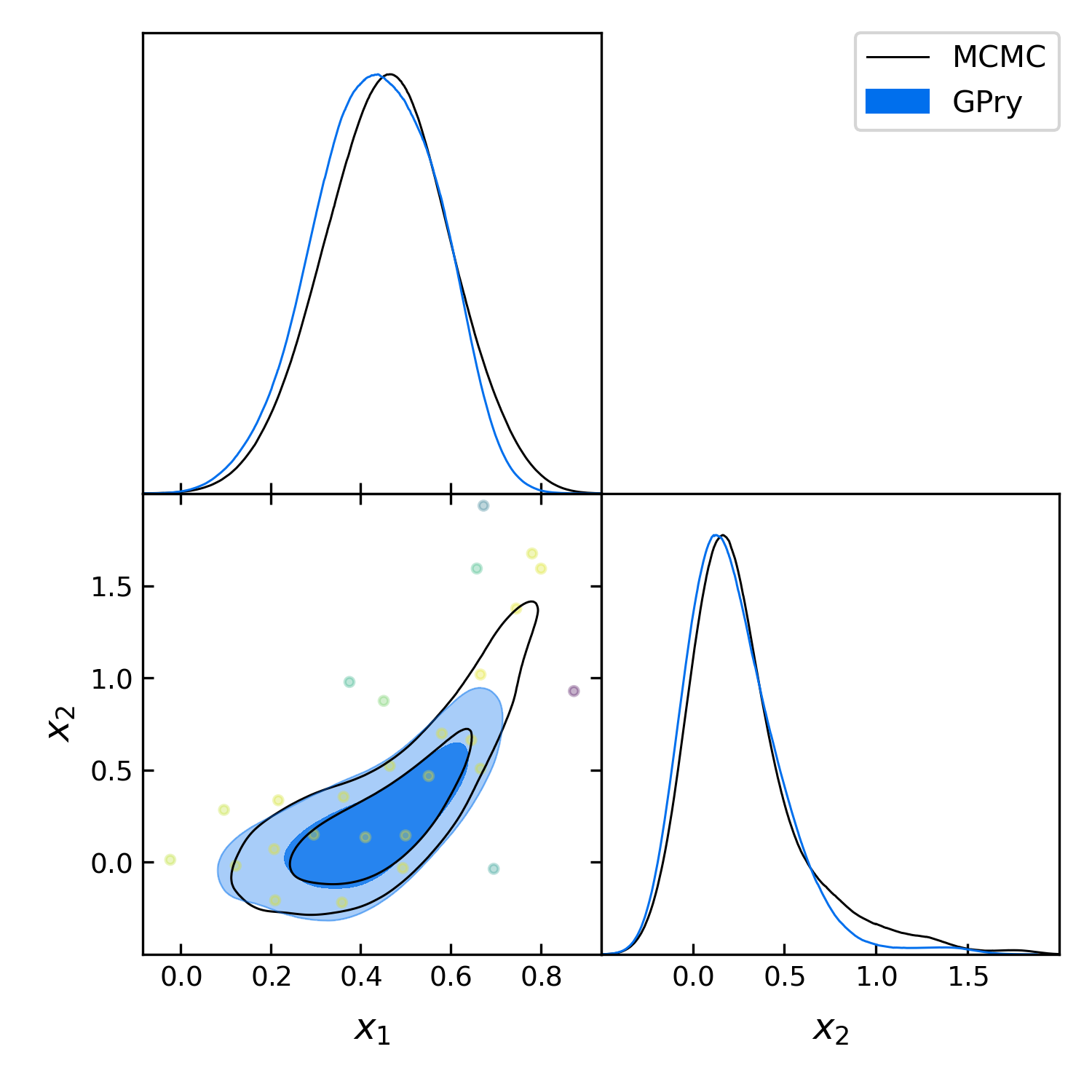
Plotting with GetDist

Finally we want to generate a triangle plot with our marginal quantities. For that we first need to extract the chains from our samplers (For both GPry and the standard MCMC) which is done in the following way:

from getdist.mcsamples import MCSamplesFromCobaya
gdsamples_gp = MCSamplesFromCobaya(updated_info_gp,
                                   sampler_gp.products()["sample"])
gdsamples_mcmc = MCSamplesFromCobaya(updated_info_mcmc,
                                     sampler_mcmc.products()["sample"])

Finally we want to generate the triangle plot to which we can add the training samples using the plots.getdist_add_training() method:

import getdist.plots as gdplt
from gpry.plots import getdist_add_training
gdplot = gdplt.get_subplot_plotter(width_inch=5)
gdplot.triangle_plot([gdsamples_mcmc, gdsamples_gp],
                     ["x_1", "x_2"], filled=[False, True],
                     legend_labels=['MCMC', 'GPry'])
getdist_add_training(gdplot, model, gpr)

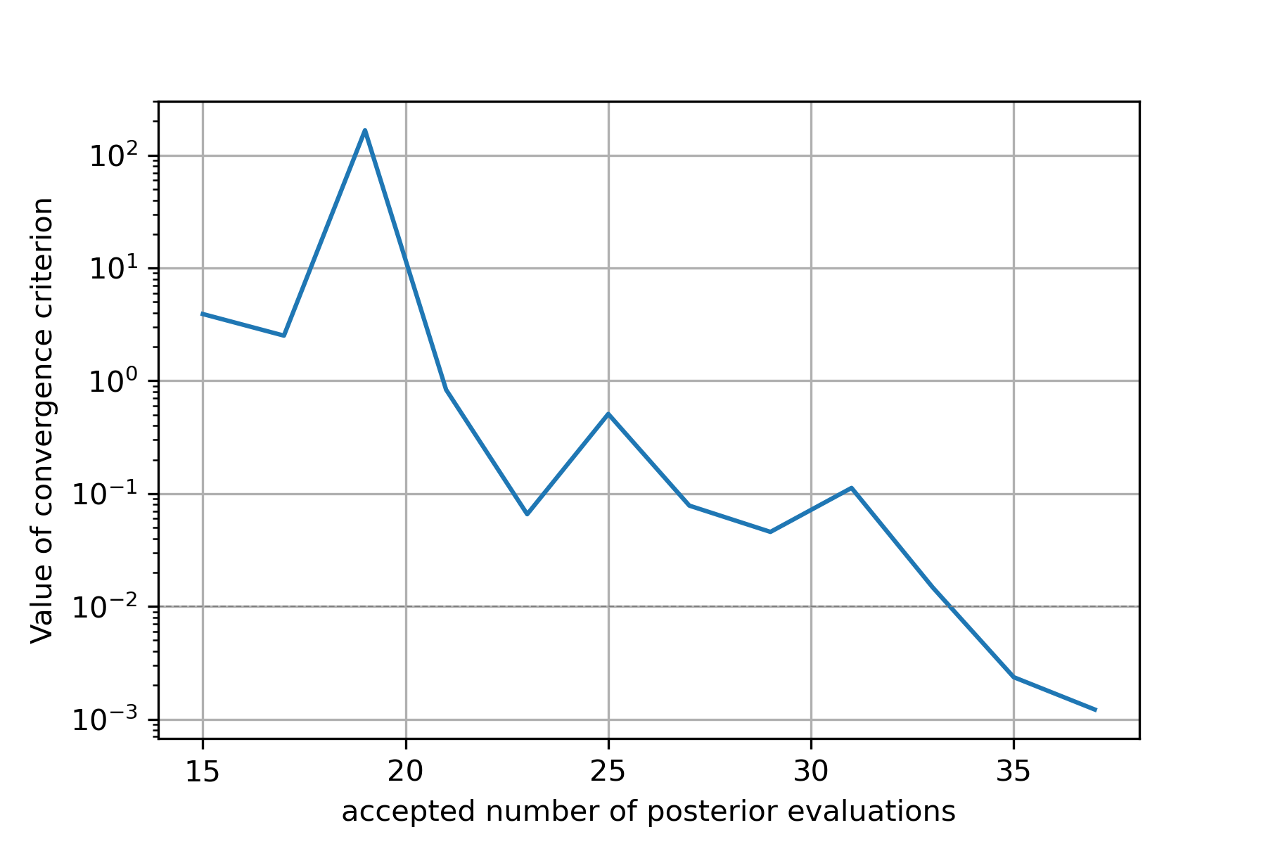
Furthermore we can simply plot the convergence history (value of KL divergence vs number of posterior evaluations) using the plots.plot_convergence() method (here we plot against the number of accepted, i.e. finite points). Note that this plot is also saved by the run.Runner when calling run:

from gpry.plots import plot_convergence
plot_convergence(convergence, evaluations="accepted")

As you can see the contours generated by GPry agree relatively well with MCMC. Furthermore you can see that the points spread apart rather far. This is due to the relatively low choice of \(\zeta\) in the acquisition function which pushes the algorithm to favour exploration over exploitation.

As expected the result is not as it would be using the standard training parameters.

Furthermore we see that the convergence criterion we chose is relatively unstable. This was to be expected though as the choice wasn’t really optimal.

The code for the example is available at ../../examples/advanced_example.py